AutoML for clinical research
Discover what IAML brings to your research.
A complete study with a few lines of Python.
Train, evaluate and explain with the built-in pipeline.
You bring the question and the data.
Can these measurements distinguish malignant from benign samples?
Scroll to follow IAML from this table to an explained prediction.
| Radius | Texture | Outcome |
|---|---|---|
| 11.25 | 14.78 | Benign |
| 14.54 | 27.54 | Malignant |
| 12.46 | 24.04 | Malignant |
Breast cancer dataset bundled with scikit-learn.
Here, 1 = malignant and 0 = benign.
IAML(...).fit(X_train, y_train)
Keep scrolling
IAML searches. Compares. Fits.
The default pipeline searches preprocessing and predictors together. IAML compares candidates by cross-validation, then fits the selected pipeline.
XGBoost
0.990Cross-validation ROC AUCCatBoost
0.995Cross-validation ROC AUCThe results become visible.
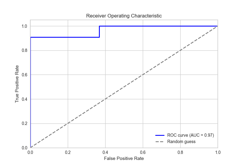
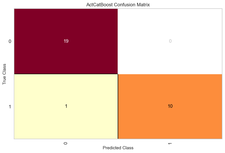
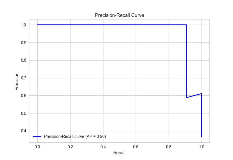
One call generates the performance figures. These use the 30 observations kept outside the search.
Balanced accuracy 0.955F1 0.952Precision 1.000Specificity 1.000Balanced error 0.045
- Prokhorenkova et al. (2017). CatBoost: unbiased boosting with categorical features. arXiv:1706.09516.
- Lundberg & Lee (2017). A Unified Approach to Interpreting Model Predictions. arXiv:1705.07874.
And the predictions become understandable.
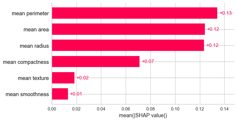
IAML computes SHAP contributions for the fitted pipeline: inspect one prediction, then compare contributions across observations.
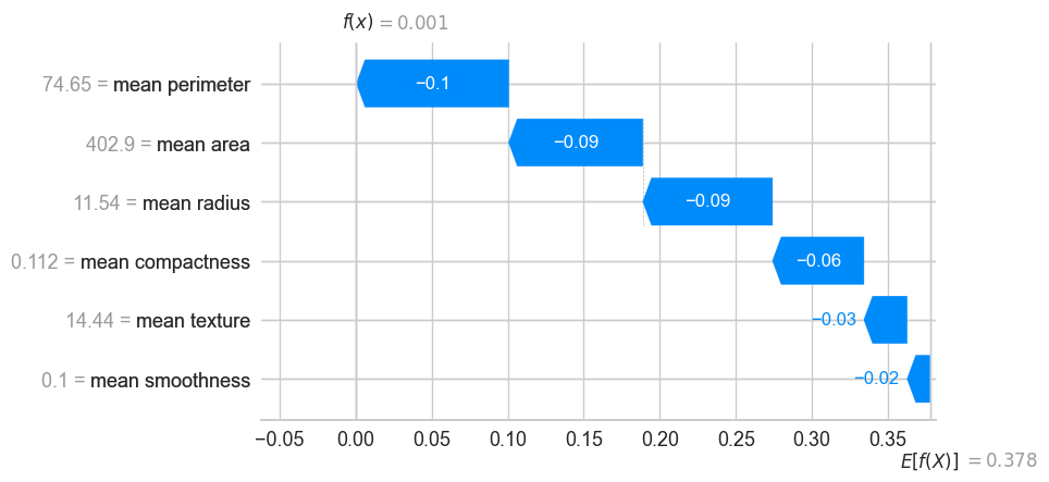
From the background average to the predicted probability of malignancy. The blue contributions lower it.
Try the complete workflow.
A fitted pipeline, performance metrics and plots, and feature explanations — connected in one Python workflow.
- Your trained pipeline
- Evaluation metrics
- Model performance plots
- SHAP explanations of predictions
- Method bibliography
IAML supports classification, regression and survival analysis.
Run the Quick Start → See the example and codeOptional customizationGo further: build your own pipeline →